Drawing arbitrary shapes with OpenGL points

Part of my Google Summer of Code project involves porting several arrow heads from Glumpy to Vispy. I also want to make a slight change to them: the arrow heads in Glumpy include an arrow body, I want to remove that to make sure you can put an arrow head on every type of line you want.

Making a change like that requires that you understand how those shapes are drawn. And for someone without a background in computer graphics this took some thorough investigation of the code and the techniques used. This article is aimed at people like me: good enough programming skills and linear algebra knowledge, but almost no former experience with OpenGL or computer graphics in general.

Implicit surfaces

The basic principle behind drawing these 2D shapes is called implicit surfaces, and it relies on a arbitrary shape function which for a given point in your image returns the distance to your shape surface or boundary from that given point. This is visualized in fig. 1.

The distances any shape function should return are highlighted in red. To actually be able to draw a shape, we need to distinguish whether a point lies inside the shape or not. We make the arbitrary decision that a negative distance lies inside a shape, and a positive distance means that the point lies outside the shape.

Distance functions for a few basic shapes

The distance functions defined below have one requirement: the center point of the shape has the coordinate (0, 0).

Circle

For a circle these distances are easily calculated:

$$ d(\textbf{x}) = ||\textbf{x}|| − r $$

Where:

• $\textbf{x}$: Vector to the point in consideration.
• $r$: The radius of the circle.

If the point lies within the circle, the length of the vector towards that point is smaller than the radius, making the distance automatically negative.

Square

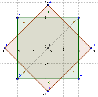
Consider fig. 2.

A square is a nice symmetric figure, so we can take the absolute values of the coordinates, and then we only need to consider the smaller highlighted square (light blue).

The distance to the boundary of the square is then:

$$ d(\textbf{x}) = \text{max}(|x_1|, |x_2|) - \frac{s}{2}$$

Where:

• $\textbf{x}$: Vector towards the point in consideration
• $|x_1|, |x_2|$ are the absolute values of the first and second element of the vector (the x and y coordinates).
• $s$: The size of the square.

Using the max function we sort of select to which boundary the distance will be calculated. Then we substract the size of the smaller square (highlighted with light blue). The resulting distance is then negative if the point lies within the square, and positive otherwise.

Combining shapes

To make more complex shapes, it is often useful to combine multiple simple shapes. To do this, we introduce some basic operations on the returned distances of a simple shape ¹.

Inverse

We made the arbitrary decision to say that the distance is negative when a point lies within the shape. To get the inverse of a shape we simply need to negate each distance value.

$$\forall x, y: \neg S(x, y) = -S(x, y)$$

Union

The union of two shapes can be retrieved by using the min function on both distance functions.

$$ \forall x, y : U(x, y) = \min(S_1(x, y), S_2(x, y)) $$

Remember that the distance value is negative when the point lies in the shape. The lowest value will win here, so if one of those distances is negative (the point belongs to at least one shape), it will return the negative value. Thus combining both shapes to a single one.

Difference

The difference of two shapes contains all points in $S_1$ excluding the points in $S_2$. This is defined as follows:

$$\forall x, y : D(x, y) = \max(S_1(x, y), -S_2(x, y))$$

Consider the example where $S_1(x, y)=−2$ and $S_2(x, y)=−1$. In short, the current point $(x, y)$ belongs to both $S_1$ and $S_2$. Using the above function for the difference, the value from $S_2$ gets negated: $−S_2(x, y) = 1$. Due to the max function, this value will win (it’s higher than -2), and therefore, it will not be part of the new shape. Which is precisely what we want, because we want all points that are part of $S_1$ but not part of $S_2$.

Intersection

The intersection of two shapes contains all points that are both part of $S_1$ and $S_2$. It is defined as follows:

$$\forall x, y: I(x, y) = \max(S_1(x, y), S_2(x, y))$$

A point will be part of the new shape if and only if both distances are negative. If one distance is positive, the max function will return this value, and a positive value means not part of the shape. This results in a shape which includes only points that are both part of $S_1$ and $S_2$.

OpenGL implementation

So how do we translate these principles to some working code? Let us first introduce some basic OpenGL concepts before throwing the shader code at you.

Shaders and drawing modes

I will not go too deep in the basics of OpenGL, but a modern OpenGL pipeline consists of multiple shaders, small programs you can write yourself. At the very minimum you’ll need a vertex shader and a fragment shader, which determine where the main “drawing points” will be positioned and the color of the individual pixels respectively. The pipeline is illustrated in fig. 3.

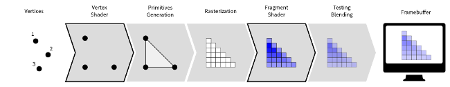
You can define your own attributes for each vertex, for example the position, colour, or orientation.

OpenGL has several modes for generating the actual primitives. These are illustrated in fig. 4.

For a more in depth OpenGL introduction, I would recommend this tutorial, Anton’s OpenGL tutorials, or opengl-tutorial.org.

Above pictures courtesy of N. Rougier²

General 2D shape shaders

For the 2D shapes we want to draw, we’re going to use the points drawing mode. OpenGL allows you to specify the point size, and the fragment shader will be called for each pixel in the point.

Let’s check the vertex shader were we position our vertices, and configure the point size.

Vertex shader

Listing 1: The vertex shader code for our 2D shapes

// Uniforms
// ------------------------------------
uniform float antialias;
uniform mat4 ortho;

// Attributes
// ------------------------------------
attribute vec2  position;
attribute float size;
attribute vec4  color;
attribute float rotation;
attribute float linewidth;

// Varyings
// ------------------------------------
varying float v_size;
varying vec4  v_color;
varying vec2  v_rotation;
varying float v_antialias;
varying float v_linewidth;

// Main
// ------------------------------------
void main (void)
{
    v_size        = size;
    v_linewidth   = linewidth;
    v_antialias   = antialias;
    v_color       = color;
    v_rotation    = vec2(cos(rotation), sin(rotation));

    gl_Position = ortho * vec4(position, 0, 1);
    gl_PointSize = M_SQRT2 * size + 2.0 * (linewidth + 1.5*antialias);
}

We first define some uniforms, attributes, and varyings. Uniforms are variables which are the same for each vertex. Attributes are variables defined per vertex, and with varyings we can pass some data to the next steps in the pipeline (for example, the fragment shader).

Each vertex has a position, and this is where our 2D shape will be drawn. The matrix ortho is used for the proper projection of the vertex to your screen. We will not explain this in-depth, but if you want to know more please refer to this tutorial on opengl-tutorial.org.

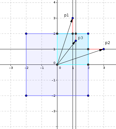
Our shapes are larger than one pixel, so we need to change gl_PointSize. Our shapes also have a size attached to them, but for the point size we scale this size with $\sqrt{2}$ (ignore the extra size for antialias en linewidth for now). We do this because our shapes can be rotated. To fit a rotated square of size x in another square, we need a bigger square of size $x\sqrt{2}$ (I hope you guys remember Pythagoras). This is visualized in fig. 5.

Furthermore, we pass along some variables to the next steps in the pipeline (size, line width, antialias, color, rotation). Note we create a direction vector for the rotation from the given rotation in radians.

Fragment shader

Listing 2: The fragment shader code

// Varyings
// ------------------------------------
varying float v_size;
varying vec4  v_color;
varying vec2  v_rotation;
varying float v_antialias;
varying float v_linewidth;

// Main
// ------------------------------------
void main()
{
    vec2 P = gl_PointCoord.xy - vec2(0.5,0.5);
    P = vec2(v_rotation.x*P.x - v_rotation.y*P.y,
             v_rotation.y*P.x + v_rotation.x*P.y) * v_size;
    float size = v_size/M_SQRT2;

    float distance = shape_func(P, size);
    gl_FragColor = filled(distance, v_linewidth, v_antialias, v_color);
}

Note we have the same varying definitions as in the vertex shader. These contain values as passed from the vertex shader. Also note the usage of the built in variable gl_PointCoord. We specified in the vertex shader the size of our point in pixels, and for each pixel in this point the fragment shader gets called. The gl_PointCoord contains the coordinates inside the point. The x and y attributes from gl_PointCoord range from 0.0 to 1.0, where (0, 0) is the bottom left corner of the point, and (1, 1) is the top right corner of the point.

There are several operations applied to these coordinates:

Step 1. First we substract $\begin{bmatrix}0.5 \\ 0.5 \end{bmatrix}$. This makes sure the origin is in the center of the point, because the distance functions we defined earlier in this article require that.

Step 2. Next we apply a rotation transformation to the point.

Remember the transformation matrix is:

$$ \begin{bmatrix} \text{cos}(\theta) & \text{-sin}(\theta) \\ \text{sin}(\theta) & \text{cos}(\theta) \end{bmatrix}$$

If you look closely at the code you see that the vector P gets multiplied with this matrix.

$$\begin{bmatrix}nx \\ ny\end{bmatrix} = \begin{bmatrix}x \\ y \end{bmatrix} \begin{bmatrix} \mathrm{cos}(\theta) & \mathrm{-sin}(\theta) \\ \mathrm{sin}(\theta) & \mathrm{cos}(\theta) \end{bmatrix} = \begin{bmatrix} x \mathrm{cos}(\theta) - y \mathrm{sin}(\theta) \\ x \mathrm{sin}(\theta) + y \mathrm{cos}(\theta) \end{bmatrix} $$

Step 3. We also scale the coordinates with v_size.

These transformations are visualized in fig. 6.

The green region in the bottom of fig. 6 is our canvas for drawing our shape. This is done by shape_func(), any function that returns the distance to the boundary of a shape as explained earlier in this article.

The filled() function determines the color for the current pixel determined by the returned distance of shape_func(). Simply put: if the returned distance is negative, it returns a color (because it’s part of the shape), otherwise it makes the current pixel transparent. It also applies some anti-aliasing techniques which I don’t know the details of, so we will not cover this in-depth.

Example: curved arrows

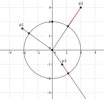
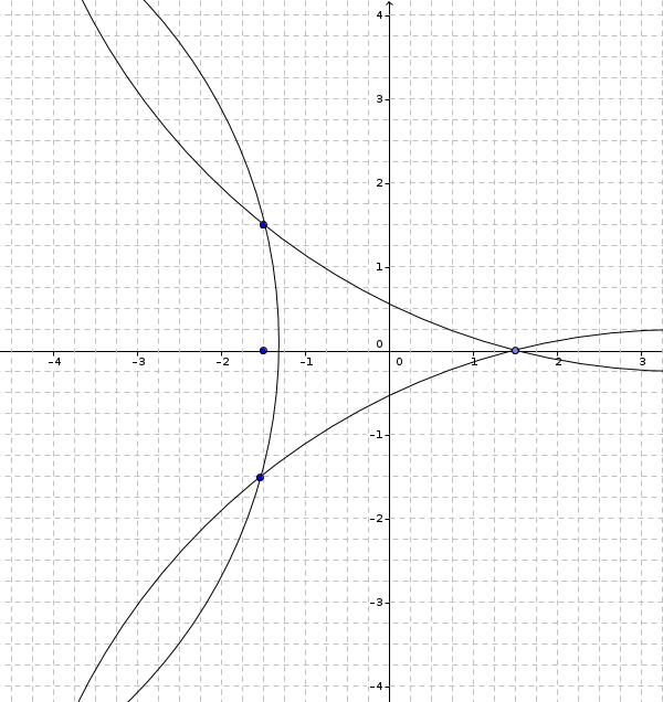
To conclude this article we will look into the distance function of a curved arrow head. A curved arrow head can be constructed using the inverse of the union of three circles. This is visualized in fig. 7, and the accompanying shader code can be seen in lst. 3.

Listing 3: GLSL function to the distance of an arrow

/**
 * Computes the signed distance to an curved arrow
 *
 * Parameters:
 * -----------
 * texcoord : Point to compute distance to
 * size : size of the arrow head in pixels
 *
 * Return:
 * -------
 * Signed distance to the arrow
 *
 */
float arrow_curved(vec2 texcoord, float size)
{
    vec2 start = -vec2(size/2, 0.0);
    vec2 end   = +vec2(size/2, 0.0);
    float height = 0.5;

    vec2 p1 = start + size*vec2(0, -height);
    vec2 p2 = start + size*vec2(0, +height);
    vec2 p3 = end;

    // Head : 3 circles
    vec2 c1  = circle_from_2_points(p1, p3, 6.0*size).zw;
    float d1 = length(texcoord - c1) - 6*size;
    vec2 c2  = circle_from_2_points(p2, p3, 6.0*size).xy;
    float d2 = length(texcoord - c2) - 6*size;
    vec2 c3  = circle_from_2_points(p1, p2, 3.0*size).xy;
    float d3 = length(texcoord - c3) - 3*size;

    return -min(d3, min(d1,d2));
}

We first define the arrow corner points as p1, p2 and p3. We use a helper function which calculates the center point of a circle through two points with a given radius r.

The distance to these circles are then easily calculated, and we use the min function to get the union of these three circles. Our arrow head is exactly the area not covered by these circles (see fig. 7), and therefore we return the inverse of this union.

References