Using locality sensitive hashing to compactly represent k-mers
K-mers are frequently used in bioinformatics to profile and compare genomes. This article describes a technique for compactly representing long k-mers with locality-sensitive hashing.

Comparing (DNA) sequences is one of the core tasks in bioinformatics, and the classic approach is to align these sequences. This is, however, a relatively slow process and not always computationally feasible, especially if you want to compare more than two DNA sequences. An alternative approach is to compare sequences based on their k-mer profiles.
A k-mer of a string is defined as any substring of of length . For example, the DNA sequence AGCGTATCGATTCA has the following k-mers if :
AGCGTATCGATTCA
--------------
AGCGTA
 GCGTAT
  CGTATC
   ...
        GATTCA
As you can see, obtaining all k-mers is easy: slide a window of size along your sequence, yielding a k-mer at each position. A sequence of length has k-mers. A common task is to count how often each k-mer occurs and compare genomes based on these counts. The main idea is that similar genomes have similar k-mer counts.
When dealing with the scale of genomes, storing counts for all these different k-mers can take up quite a lot of memory. First, the number of distinct k-mers grows exponentially with the length of . In the case of DNA sequences, our alphabet size is 4: A, C, T, G. Therefore, there are possibilities of length . The value of depends on your application and organism, but values ranging from 5 to 32 are common.
Next, think how we would store the k-mer itself. We could store each letter as ASCII character, requiring 8-bits per character. However, this is a bit wasteful because we only have four characters in DNA. An optimisation would be to use 2 bits per character: A=00, C=01, T=10, G=11. This would allow us to store a k-mer of length 32 in a 64-bit integer. Still, this may not be good enough. I’ve seen cases for where it went up to more than 100 GB, and that’s quite a lot of memory even if you have access to a decent compute cluster.
This post will explain a technique described in the paper by Cleary et al. for to reduce the memory consumption for storing k-mers. The main insight is that we often don’t need the exact count of each k-mer, and can take some shortcuts by missing some k-mers. Because of the exponential number of different k-mers and because genomes are often large, missing a few k-mers will not have a huge impact. Furthermore, when dealing with whole genome sequencing datasets, we must also deal with sequencing errors and expect some k-mers to be false. In a lot of cases, using approximate k-mer counts is appropriate.
We start by transforming each k-mer to a complex vector, using the following encoding:
A k-mer is now a vector of length , where each element represents a DNA base as a complex number. A k-mer is now a point in a k-dimensional space. Notice that similar k-mers will be “neighbours” in this k-dimensional space. This is not an efficient encoding, but we can apply a few smart operations to convert this to a smaller integer.
The idea is to divide our k-dimensional space into a lot of bins. This can be done as follows: generate a random complex vector of length k, which can then be interpreted as the normal vector of a plane through our k-dimensional space. This plane divides our space in half: certain k-mers lie on the “left” side, while other k-mers lie on the “right” side of this plane. See the figure below for an example. If we note a zero when the k-mer lies on the left and a one if on the right, we obtain a bit value.

Repeat this n times, and you obtain n bit values. For example, we could store the result from drawing 32 random hyperplanes in a 32-bit integer. Note that we split the space in half each time we draw a random hyperplane, creating bins in our -dimensional space.
It is possible, however, that two distinct k-mers end up in the same bin and thus have the same 32-bit integer value (if =32). We can actually calculate the probability of such an event. Recall that our k-mers are just ordinary complex vectors and that similar k-mers are neighbours in the k-dimensional space. We can compute the cosine of the angle between the two vectors as follows:
Here u and v are two k-mers in our complex k-dimensional space. The probability of these two k-mers being in the same bin, is equal to the probability that no random hyperplane cuts through the angle of u and v. This is visualised in the figure below.

We end up with the following equation:
Here, represents the hash value of a k-mer u, or the n-bit integer by generating random hyperplanes.
This is the reason why this could be used for approximate counting of k-mers, because some k-mers may be mistaken for another. By tuning and you can try to minimize the impact on your application. The effect is even further minimized because similar k-mers have a higher probability of ending up in the same bin than dissimilar k-mers, while reducing the number of bits you need to store the k-mer.